Part 0: Image Sharpening
Image sharpening is one of the most basic functionalities of any image editing program, like Adobe Photoshop.
We often use it to make our images clearer and our edges cleaner. But what exactly does Photoshop do, when we tell
it to sharpen our latest vacation photo?
To sharpen an image, we basically follow the formula: img + α * highpass(img),
where highpass(img) is the high pass version of our original image, and α is a constant.
To get the high-pass-filtered version of an image, I convolved each color channel of the photo with a
Gaussian kernel of specified size and σ. The right σ to use often depends on the
particular image's unique attributes (it's size, resolution, etc). I often changed the sigma depending on
the image's size (a larger sigma for larger images, and vice versa). I specified my Gaussian kernels to be
6*σ x 6*σ squares. α, on the other hand, determines how much of an effect your high-pass-filtered
image will have on your original image. In other words, the degree to which you would like to sharpen you image.
You'll notice, from the images below, that as α increases, the photo takes on a more processed, artificial appearance.

Original Image
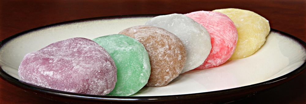
α = 0.5; σ = 6

α = 1; σ = 6

α = 2; σ = 6
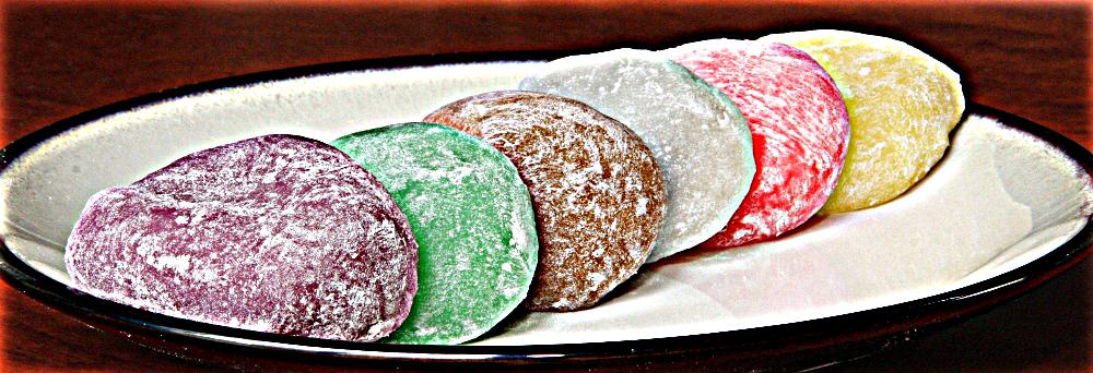
α = 4; σ = 6
α = 6; σ = 6
Part 1: Hybrid Images
Look carefully, what do you see? Now, look harder....
Knowing how to high-pass-filter an image means we also know how to get
the low pass version as well! Essentially: lowpass(img) = img - highpass(img).
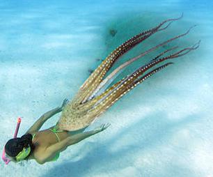
Using these skills, we can now create "hybrid images," that is, static images
that change in interpretation as a function of the viewing distance. This just
means that people who look at the picture will see one thing when
they're close to the image, and another thing when they're farther away.
Hybrid images work because high frequency dominates human perception at
shorter distances, while low frequency dominates perception at greater
proximities. This is in part due to the fact that humans, unlike hawks, for instance, have no
need to see farther things exceptionally clearly. For us, what matters most
is our immediate surroundings. We'll take advantage of this human trait in
our construction of hybrid images.
A BASIC RECIPE FOR HYBRID IMAGES:
Choose two images you'd like to combine. Let high_img be the
image you want to be visible at close distances, and low_img be
the image you want people to see when they're farther away.
        1. Align high_img and low_img, and save those as aligned_high and aligned_low
        2. high = the high-pass-filtered version of aligned_high
        3. low = the low-pass-filtered version of aligned_low
        4. Hybrid image = avg(high, low)
It should be noted that the alignment of the two images is very important
in producing a good hybrid image. As noted in the Hybrid images paper,
lack of alignment can cause the two images to interfere with each other in ways
detrimental to the viewier experience. The best situation is one in which the
low pass image is masked by the high pass image at close proximity, meaning that
the two images are very well aligned. In this case, I manually aligned the images
each time, and chose two points in each image that corresponded to each other.
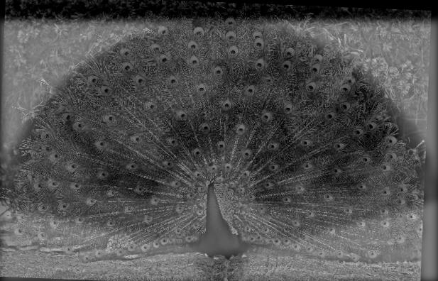
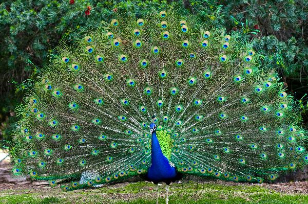
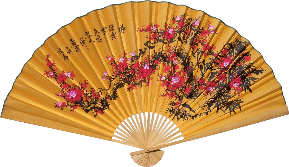
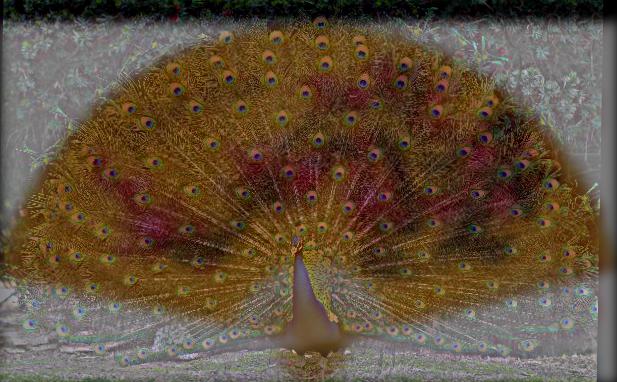
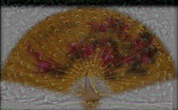
Analysis of a Hybrid Image: Peacock and Fan
In building this hybrid image, the peacock was my high pass image, with σ = 6.
The fan was the low pass image with σ = 6. I decided to keep the σ's the same
because both images are similar in size. Before proceeding, both images were manually aligned
and reduced to grayscale.
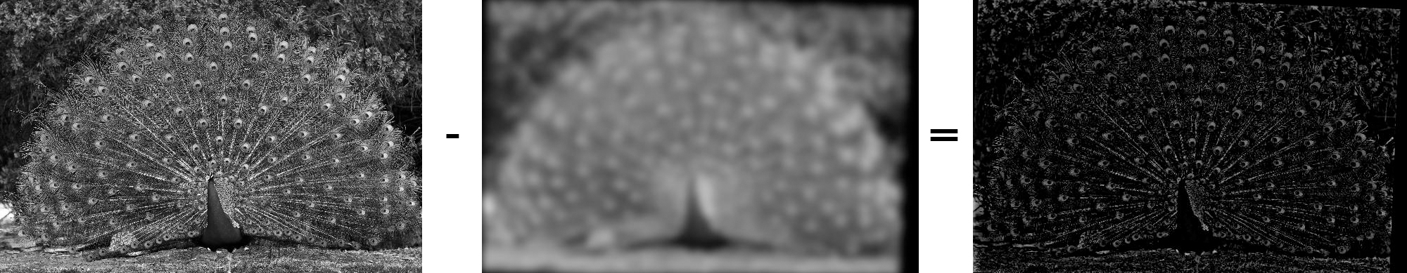
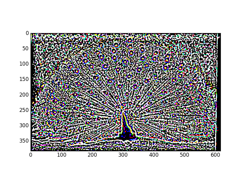
To construct the high pass image, I, in accordance with the procedure given above,
took the original grayscale image and subtracted a low pass version of the image
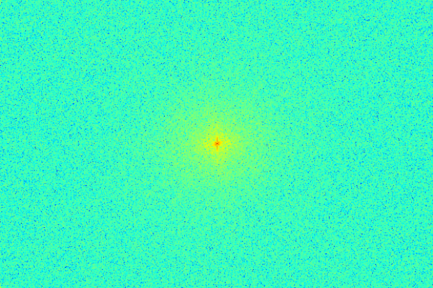
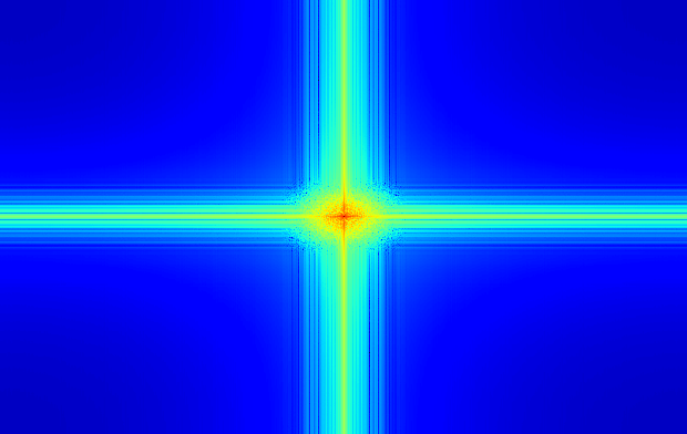
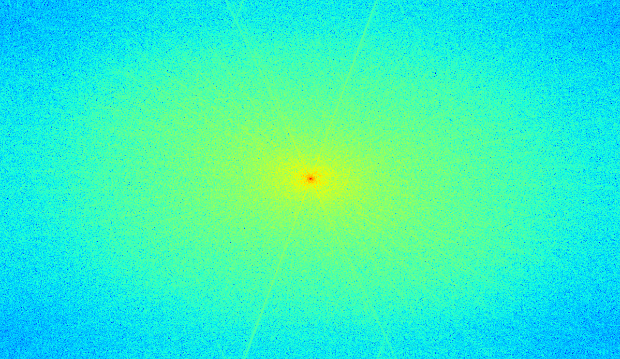
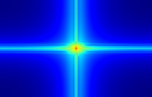
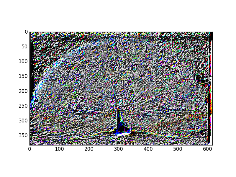
from it in order to obtain the high pass peacock. The FFT frequency graphs of these
images are given below, each placed below its respective image:
The darker colors indicate lower frequencies. Notice how the high frequency FFT
diagram is the brightest, most of the lower frequencies having been removed
from the subtraction.
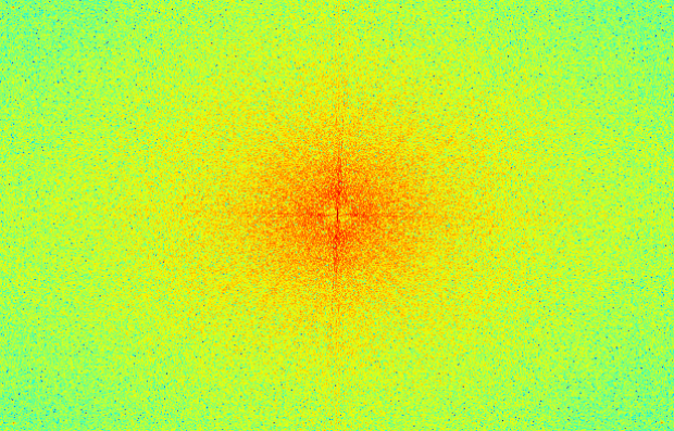
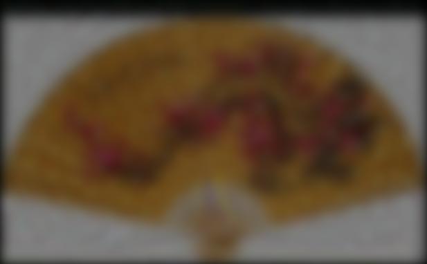
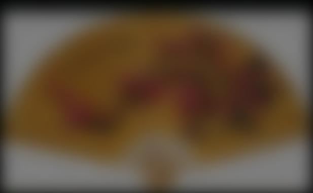
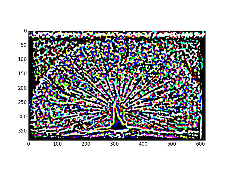
To obtain the low frequency version of the fan, I convolved the original image
with its respective Gaussian kernel. Since σ = 6, the kernel was 36 by 36 in size.
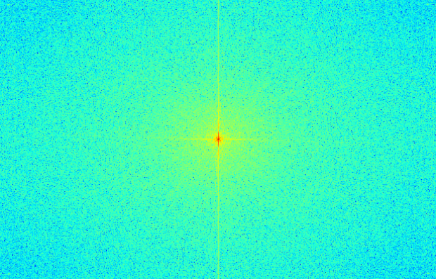
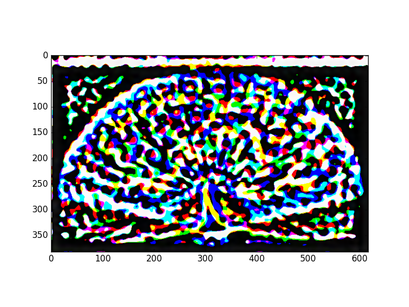
From the FFT images below, it can be seen that the original image, which was
full of high frequencies was largely reduced to low frequencies by the Gaussian filter.
FFT of original fan image
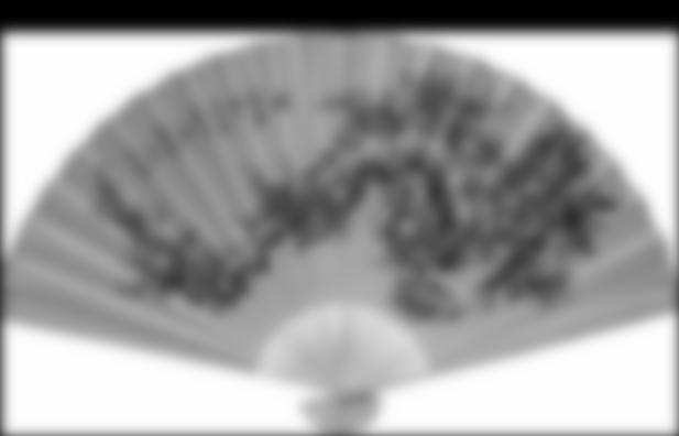
Low pass fan
FFT of low pass fan
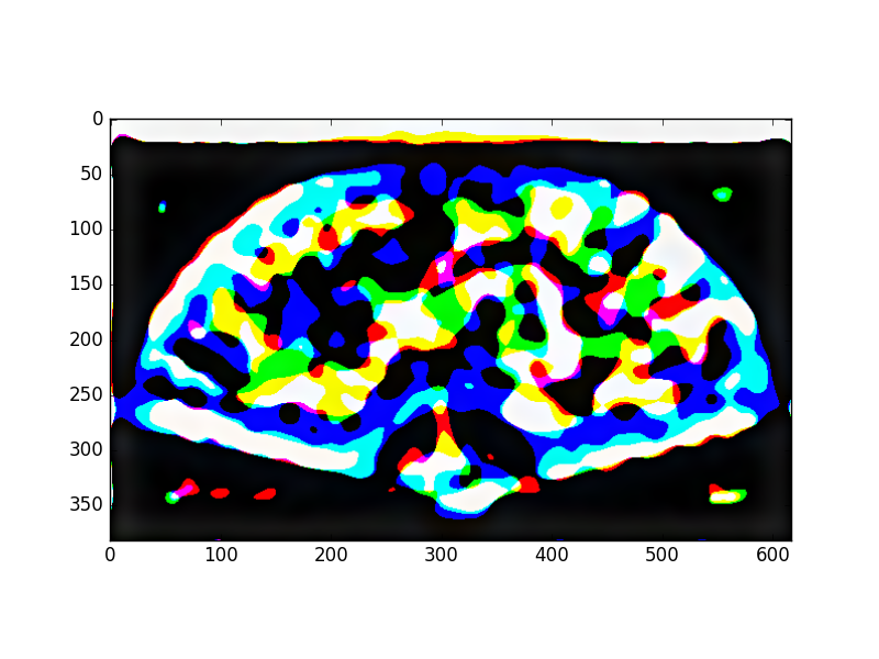
Above is the final hybrid image, along with its FFT diagram.
More Hybrid Images
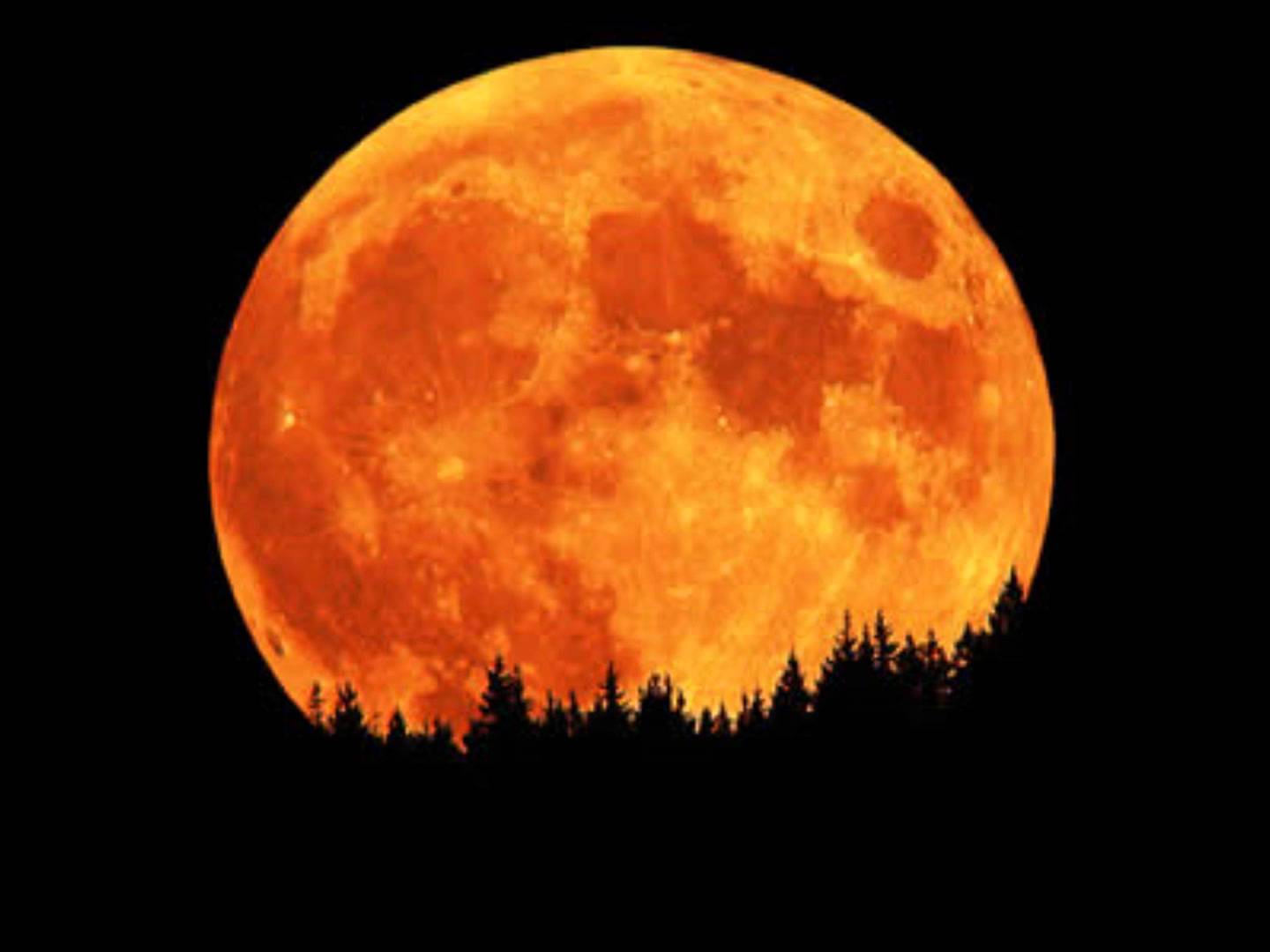
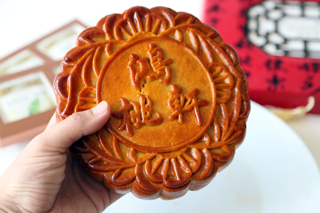
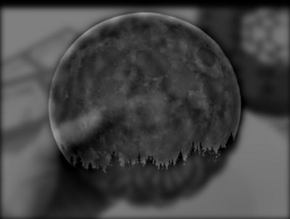
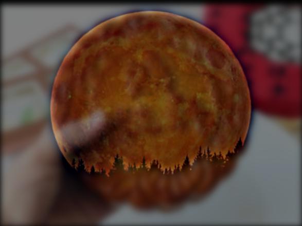
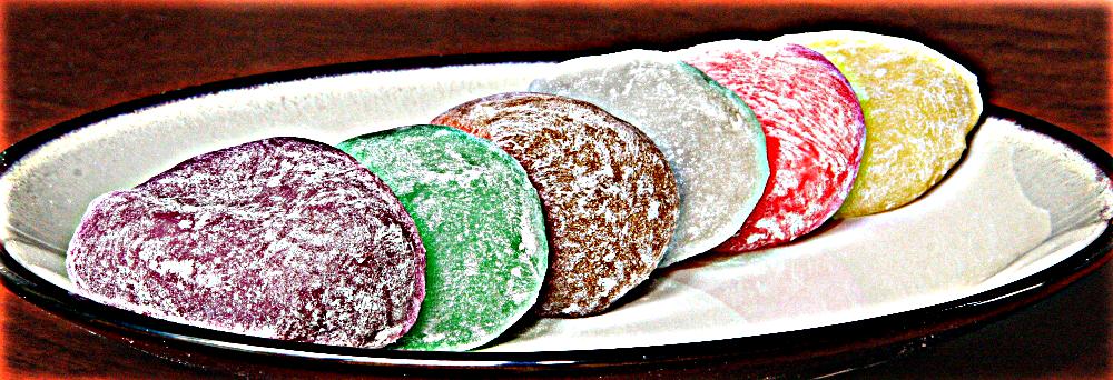
HARVEST MOON & MOONCAKE
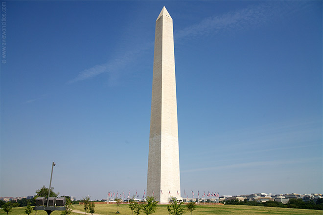
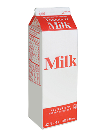
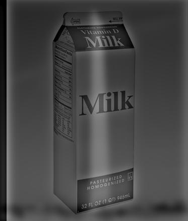
FAILURE CASE: MILK & WASHINGTON MONUMENT
This particular case likely did not work out because of the drastic visual
differences between the milk carton and the monument. One is shorter and wider,
while the other is taller and thinner. In accordance with the research paper's
point about proper alignment, the milk carton is not compatible with the monument
in that they can't be properly aligned. This results in the images interfering with
each other and distracting the viewer. Thus, the output is sub-optimal.
Bells & Whistles: Colored Hybrid Images
Part 2: Stacks
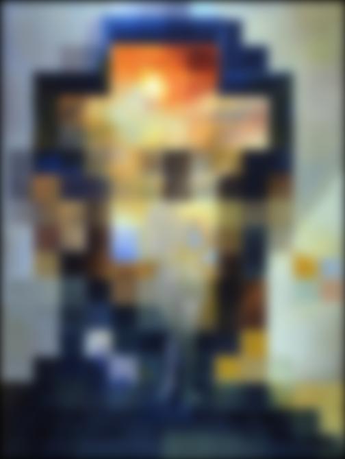
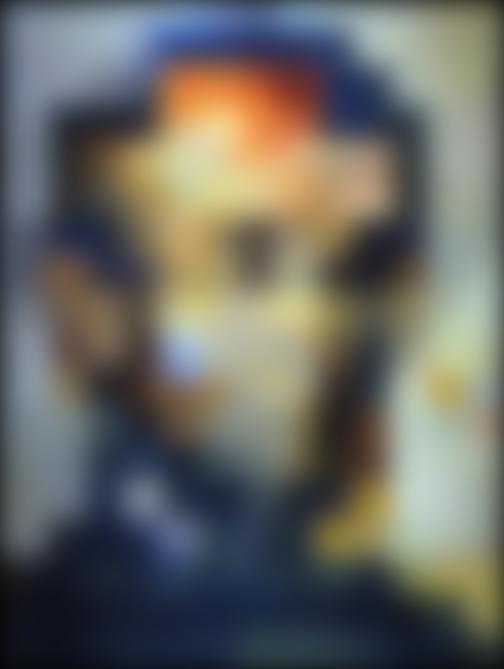
Stacks for Salvador Dali
Gaussian Stack
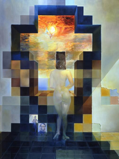
Original
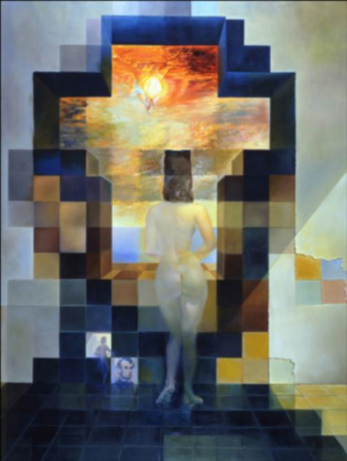
σ = 1
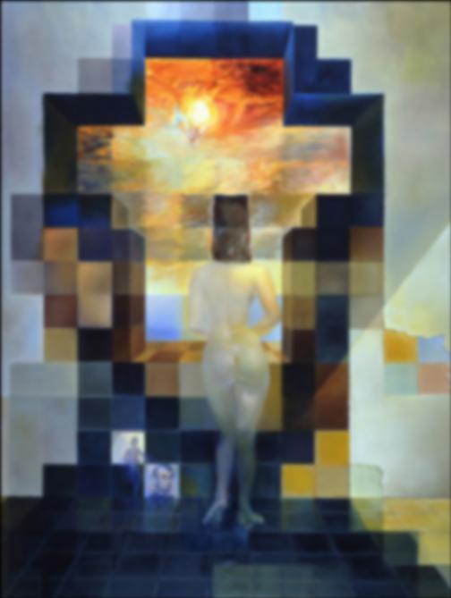
σ = 2

σ = 4
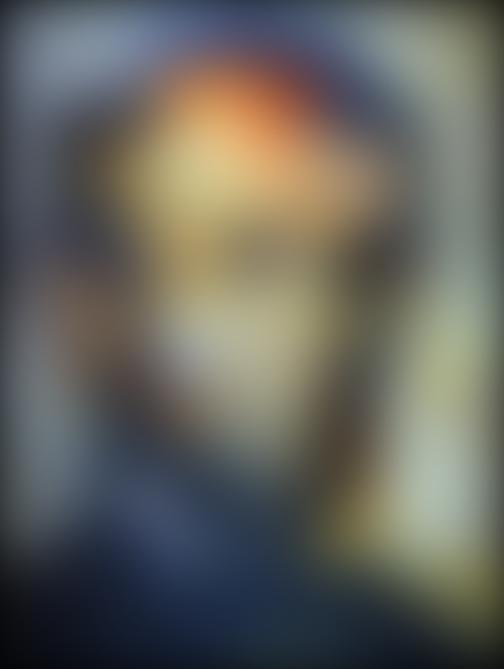
Laplacian Stack
g0 - g1
g1 - g2
g2 - g3
g3 - g4
Stacks for Peacock and Fan
Gaussian Stack

Original
σ = 1

σ = 2

σ = 4
σ = 8
σ = 16
Laplacian Stack
Original
σ = 1
σ = 2
σ = 4
σ = 8
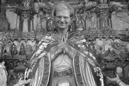
Part 3: Multiresolution Blending
Grayscale Blending
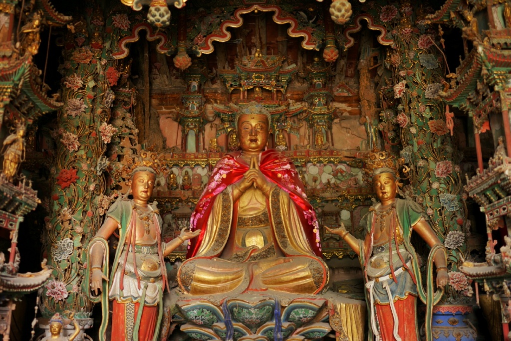
ORIGINAL IMAGES
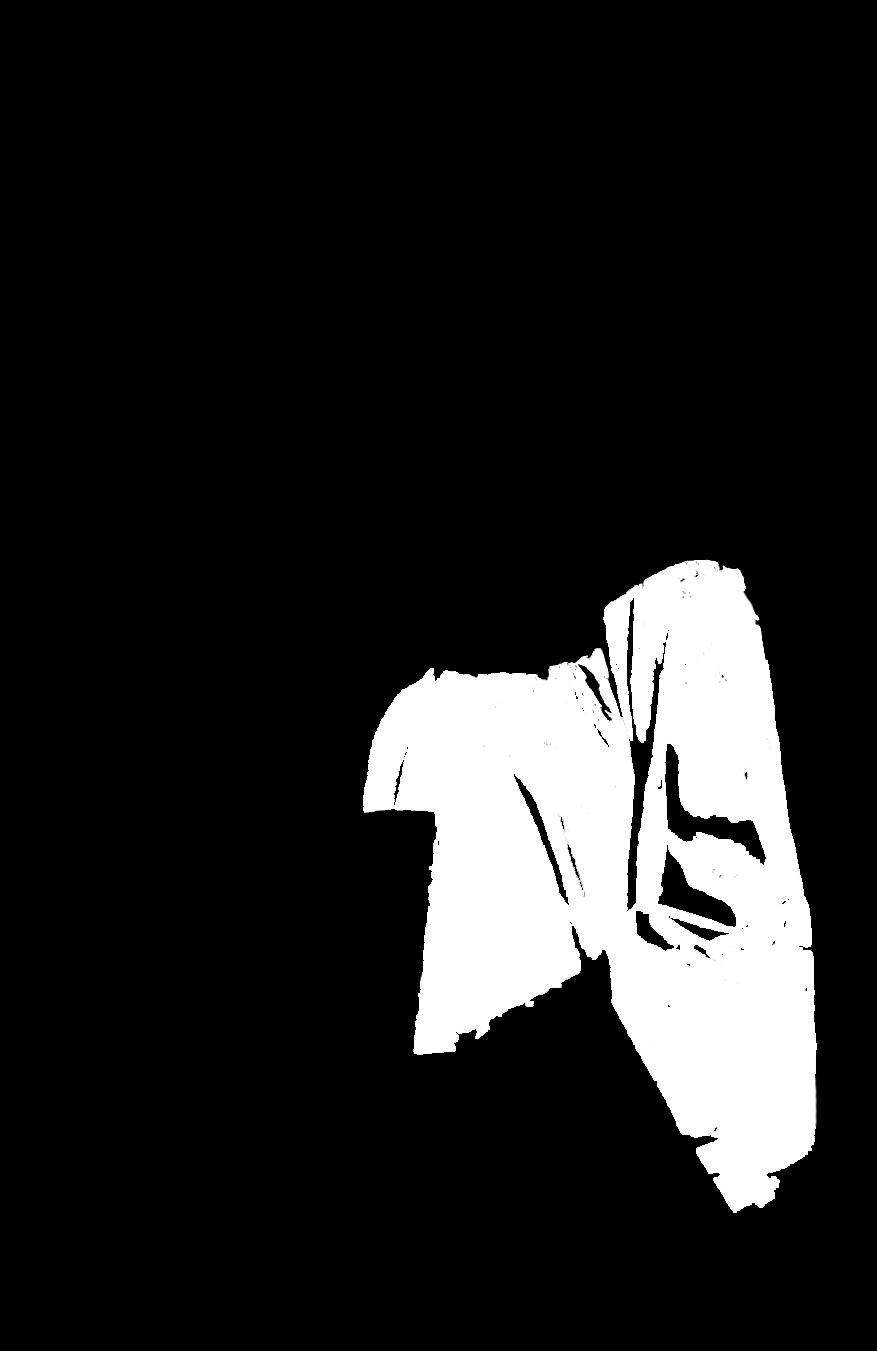
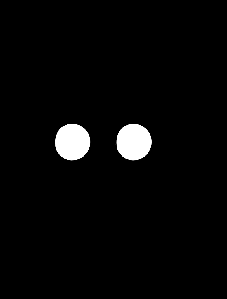
HOW IT WORKS
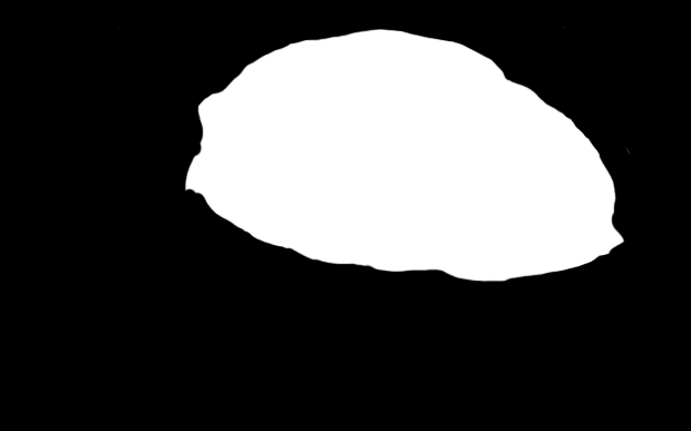
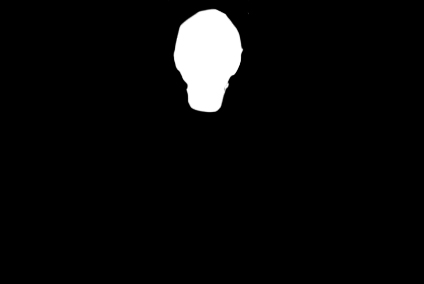
Multiresolution blending works by taking two images that you want to blend,
and creating a black and white "mask." The mask will be white where you want
the first of your images to appear in the final blended output, and black where
you'd like the second image to appear. In this case, I created a mask that
matched the head of the statue to Professor Efro's face.
The general procedure is to take in two images. Let's say that img1 corresponds to
the white areas of the mask, and img2 corresponds to the black areas. Here's a high-level
recipe for blending the two pictures:
        1. Make a Laplacian stack for img1 (L1)
        2. Make a Laplacian stack for img2 (L2)
        3. Make a Gaussian stack for the mask (Gm)
        4. For each level i of the stacks for all the images, find:
            Gm_i * L1_i + (1 - Gm_i) * L2_i
        5. Blended image = sum of all Gm_i for all levels i
The number of levels is arbitrary and completely up to you. My images
used levels of 6.
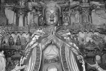
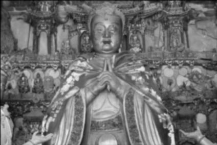
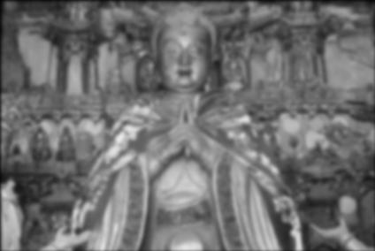
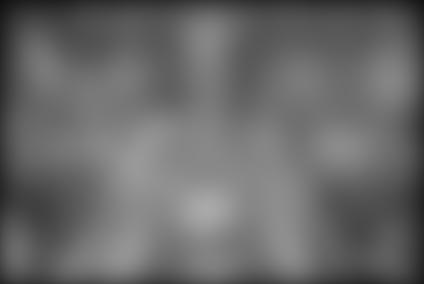
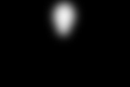
GAUSSIAN STACK OUTPUT
To create the Efros Statue image, Gaussian stacks of six levels were generated for each component image.
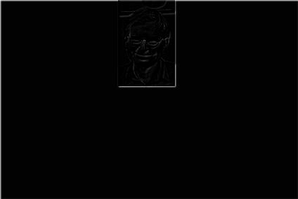
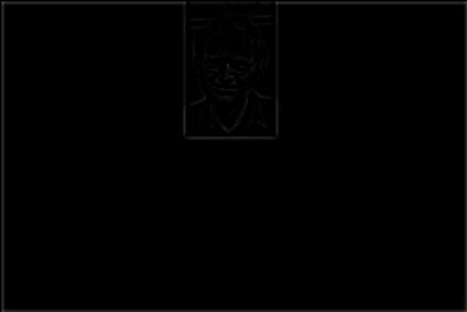
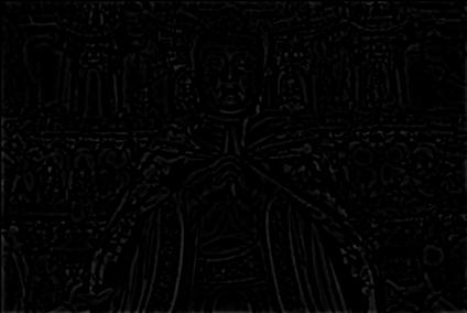
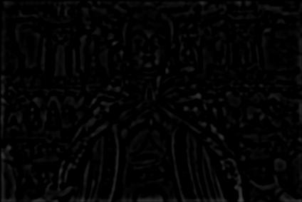
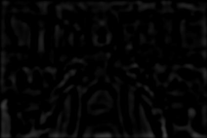
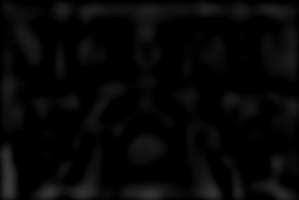
LAPLACIAN STACK OUTPUT
Laplacian stacks of five layers were also generated for two non-mask images.
The following is the Laplacian stack generated for the statue image.
Note that the very last image in each stack is always the last image from
the corresponding Gaussian stack.
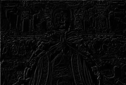
Combining all the Laplacian and Gaussian stack outputs in accordance with the
formula specified above, results in the blended Efros Statue image!
Bells and Whistles: Adding Color
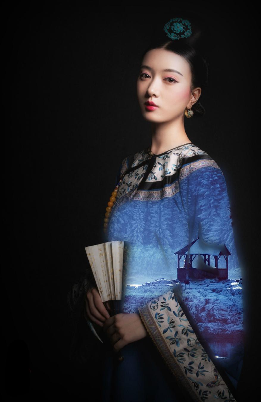
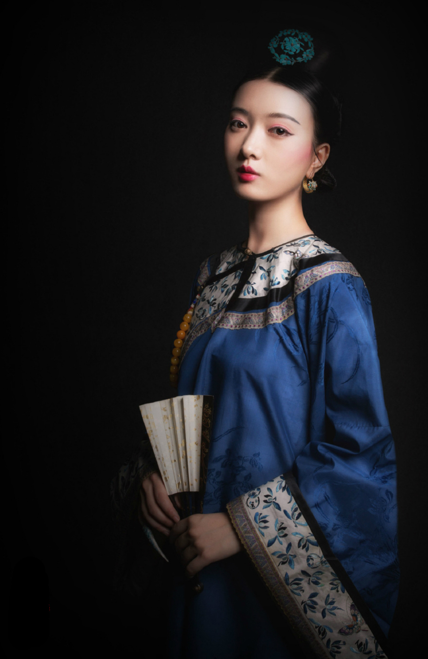
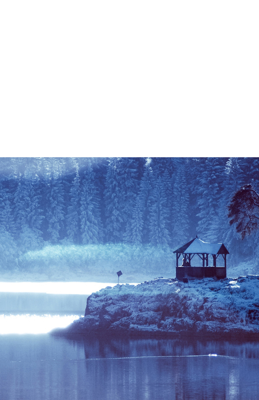
FOREST ROBES
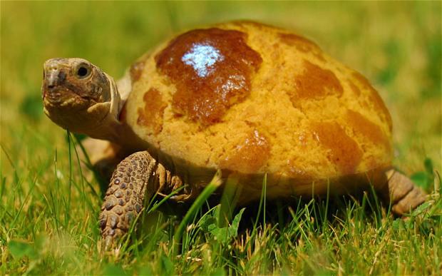
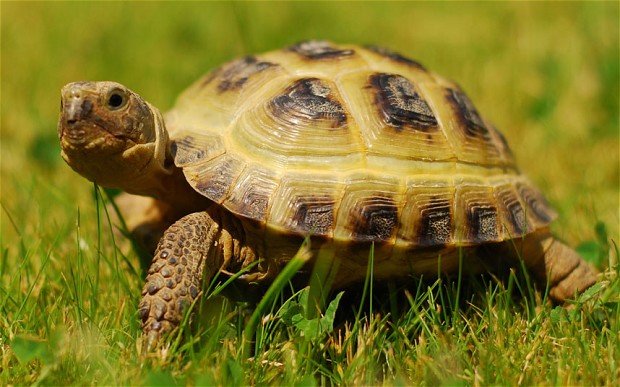
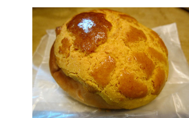
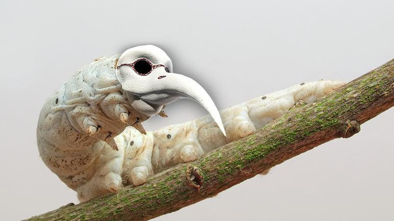
TURTLE-PINEAPPLE BUN
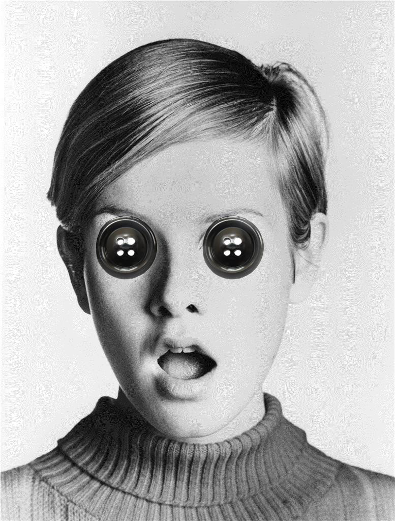
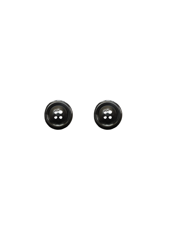
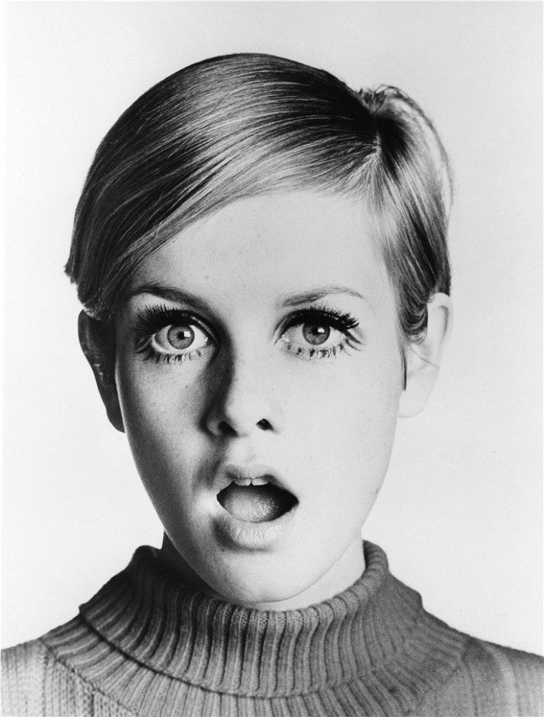
BUTTON EYES
FAILURES
I found that blending images with fairly different color schemes or textures
often did not produce optimal results. Ultimately, the more similar the images,
the better the result of the blend.