PART 1: Creating Panoramas by Hand
This project concerns programmatically taking a few related images, warping them to the same point of view, and then piecing them together into a large composite image. Such techniques are often seen implemented in products that involve the creation of panoramas or wide angle lenses.
I. CALCULATING HOMOGRAPHIES
In order to correctly warp an image A to image B, we first need to calculate the homography matrix between them. A homography can tell us the position of a pixel in image A when warped to the plane of image B.
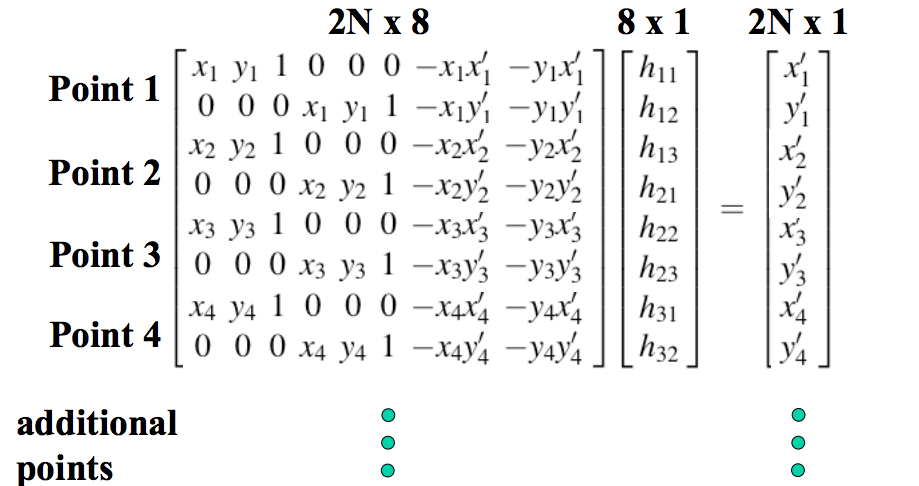
Generating a homography requires at least four points, because we need to solve for eight unknown variables. In this project, I manually selected corresponding points between the two images, but there are techniques out there that will allow you to programmatically generate such points as well. I then solved a system of equations much like the following:
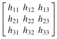
The elements of vector h are also the elements of the square homography matrix H, which can be constructed as specified below. For our purposes, h_33 is 1.
II. IMAGE RECTIFICATION
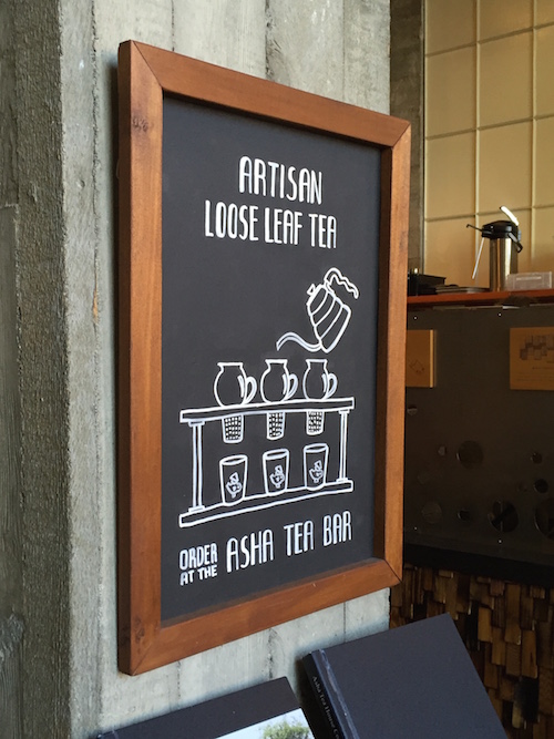
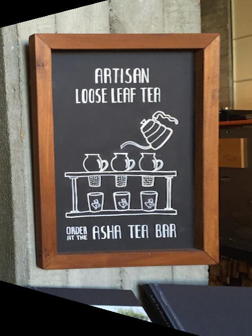
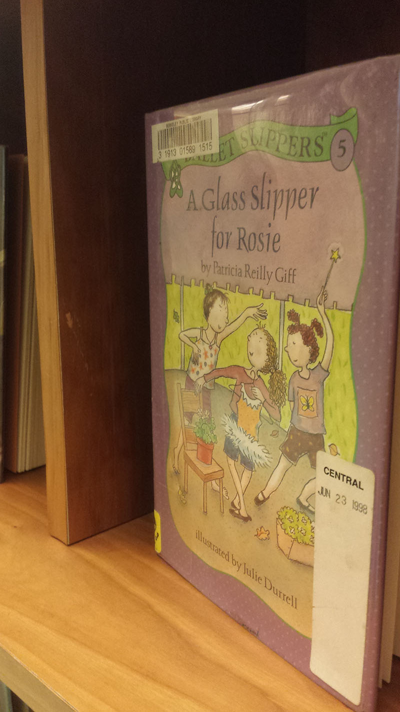
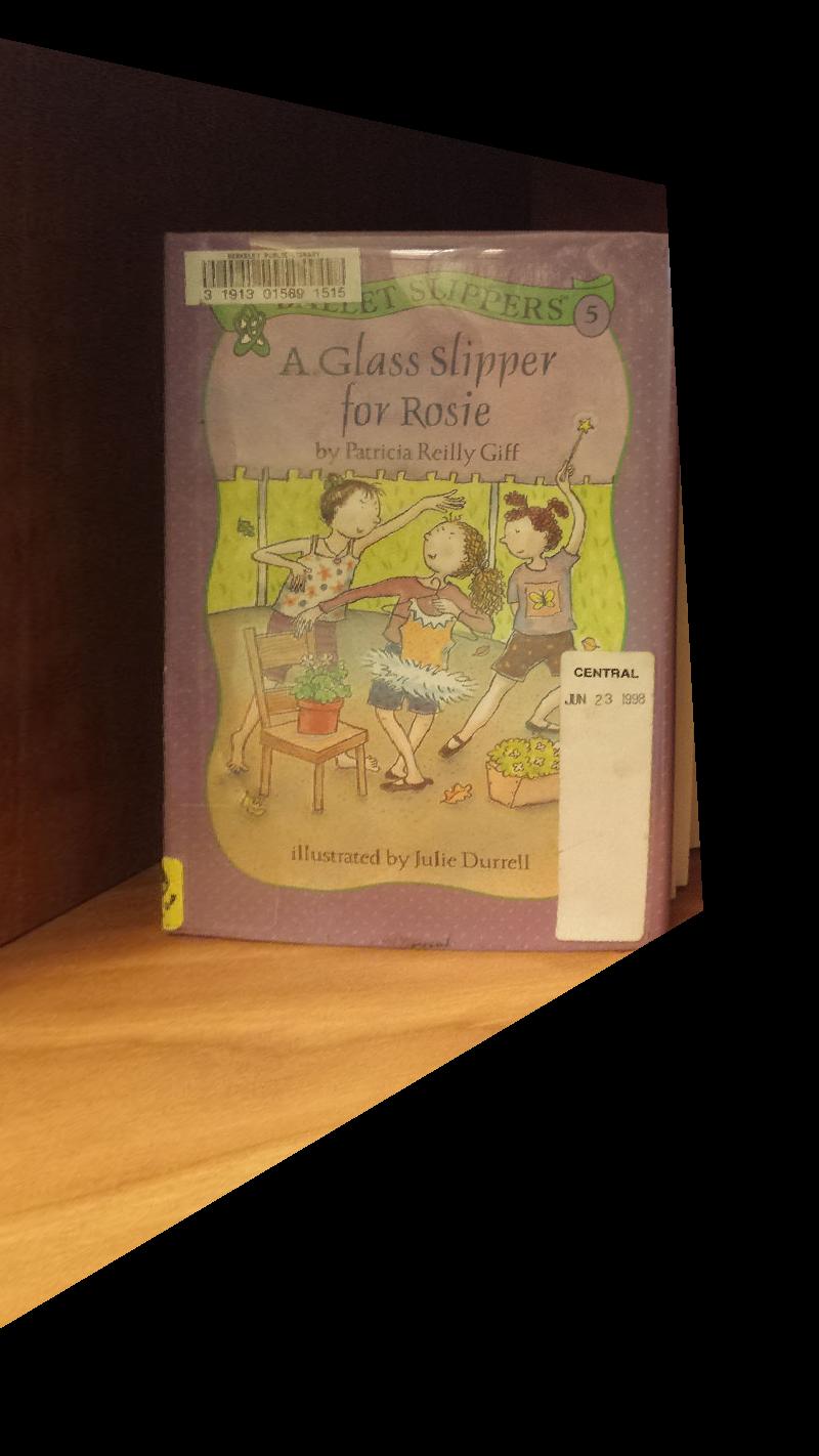
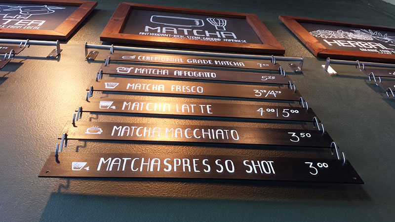
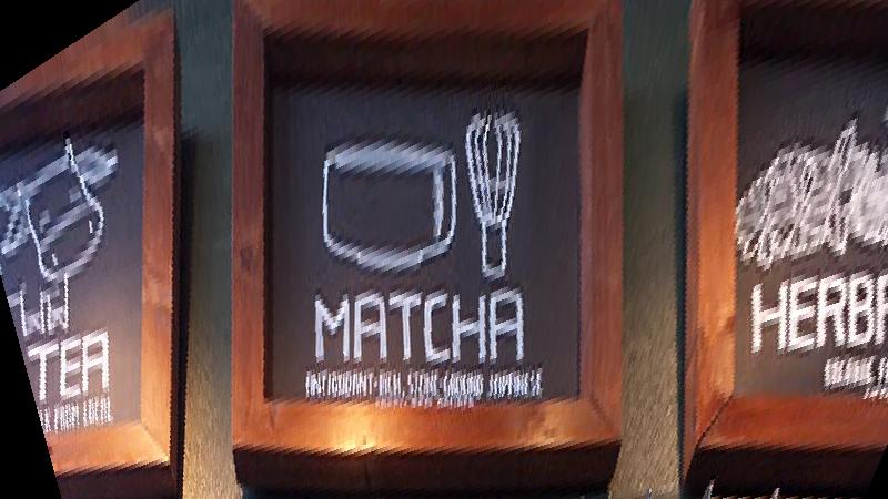
Using the above technique for finding a homography between two images, we can now essentially take any image we want and warp it to match a desired point of view. Below are examples of instances where I took an image and warped various signage / planar objects to face forward.
III. MOSAIC CONSTRUCTION
Now that we know how to warp and rectify images, we can use these same techniques to stitch many images together to create a panorama! I used sets of three images to create my mosaics.
First, we can determine the size of the final panorama by doing forward warping on the left corners of the left image and the right corners of the right image. Simple arithmetic allows us to use this information to find the width and height of the panorama canvas. Forward warping also allows us to figure out the coordinates of the rest of the corners of our images when mapped onto the plane of the final panorama. This information is useful for finding the sizes and locations of overlapping areas between the three photos.
With this information, we can now warp the images towards a plane of our choosing. I decided to warp the left and right images to the plane of the center image. If a point in the final panorama applies to more than one image (Ex. This would happen if the same flower shows up in the left and center images), I used weighted averaging to smooth out the difference. I detected overlaps using calculated information about the left and right bounds of each intersecting area between the images.
To find the weights for linear blending between, say, the left and center images, I used the ratio between the current point’s distance from the left edge of the intersecting area and the total width of the intersecting area. Subtracting that value from 1 gave me the weight for the pixel value from the center image.
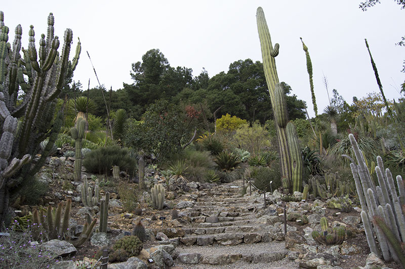
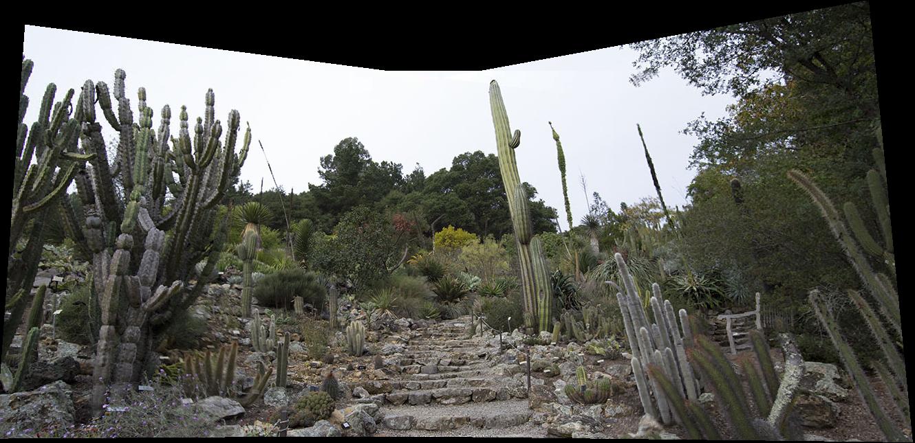
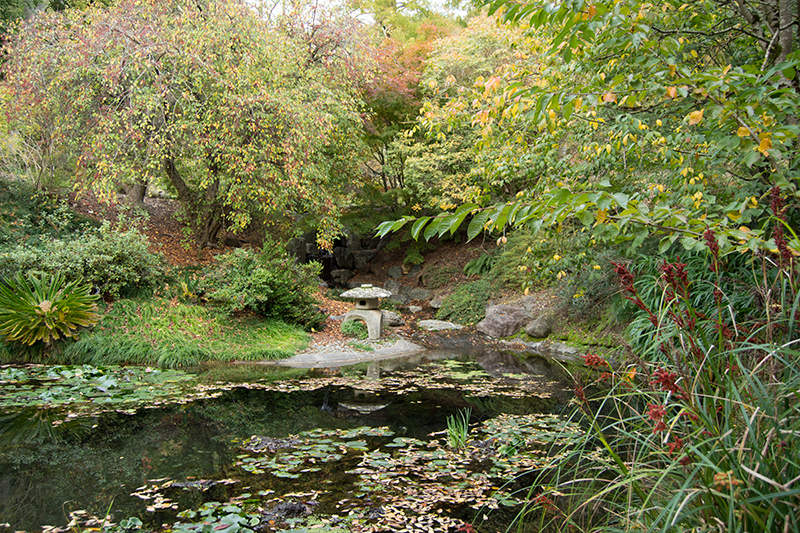
To take photographs for this project, I paid a visit to the Berkeley Botanical Gardens and used a tripod to ensure that all my images were coming from a fixed point of rotation. Featured below are some of my results:
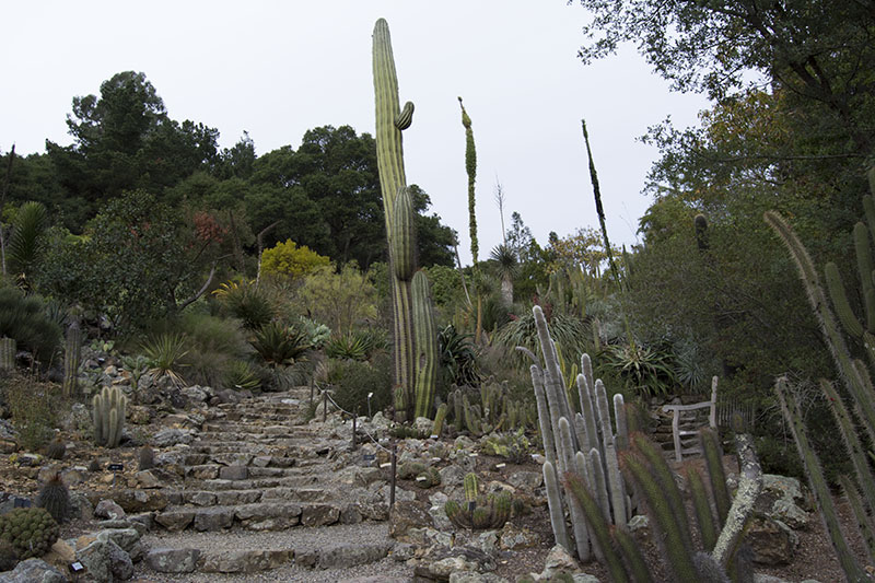
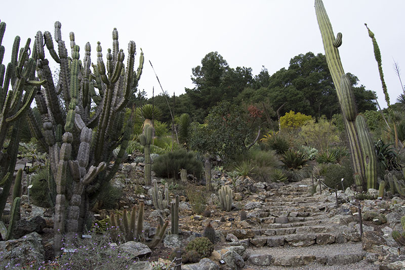
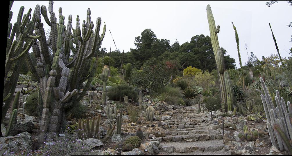
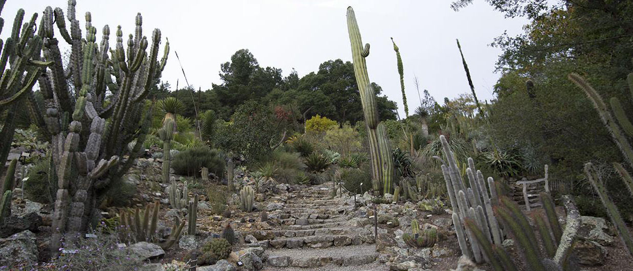
MOSAIC EXAMPLE 1: DESERT ECOSYSTEM
This one actually turned out better than I expected (likely because I managed to keep the brightness consistent between shots).
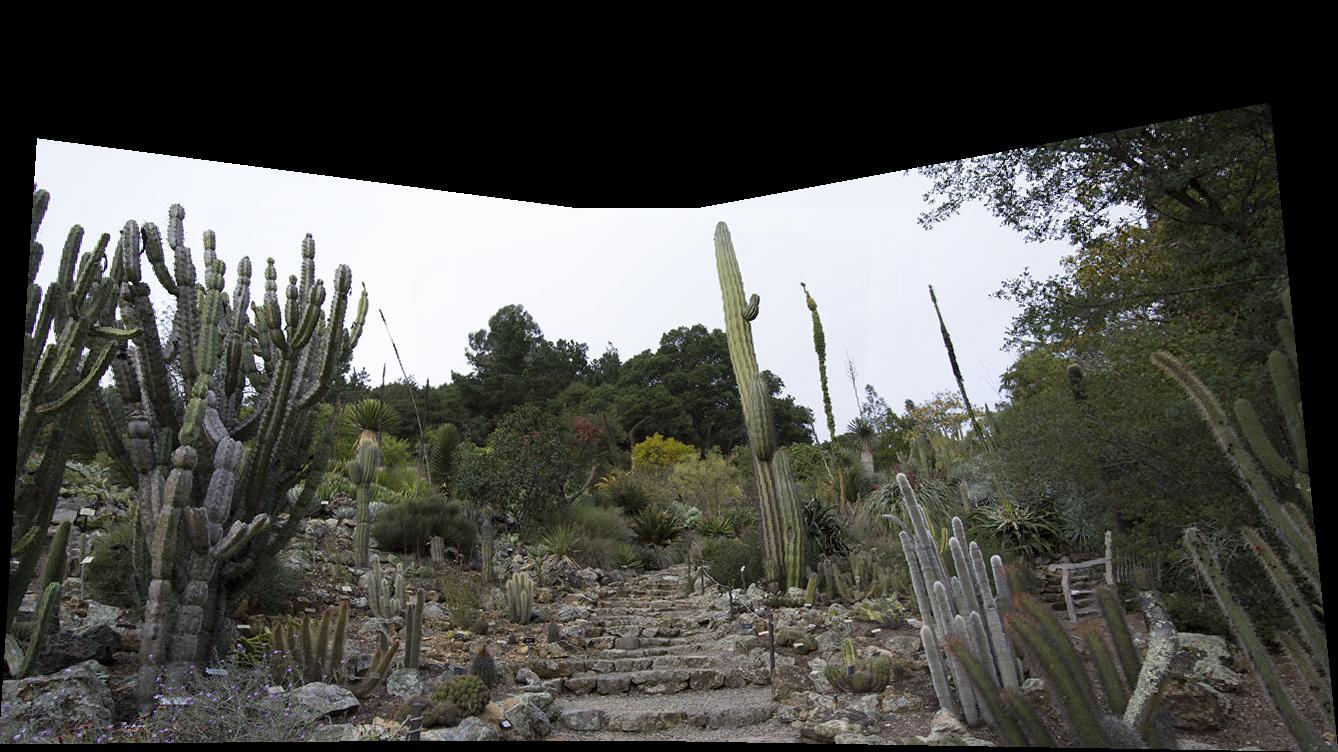
Linear blending
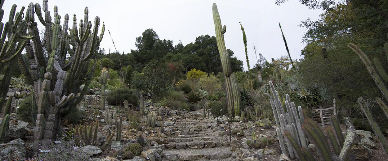
Cropped for aethetic effect
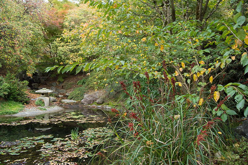
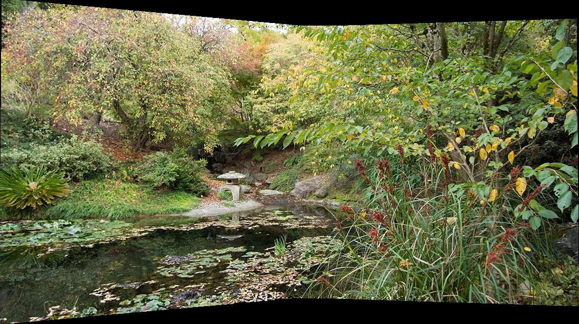
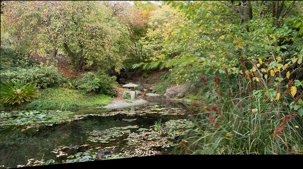
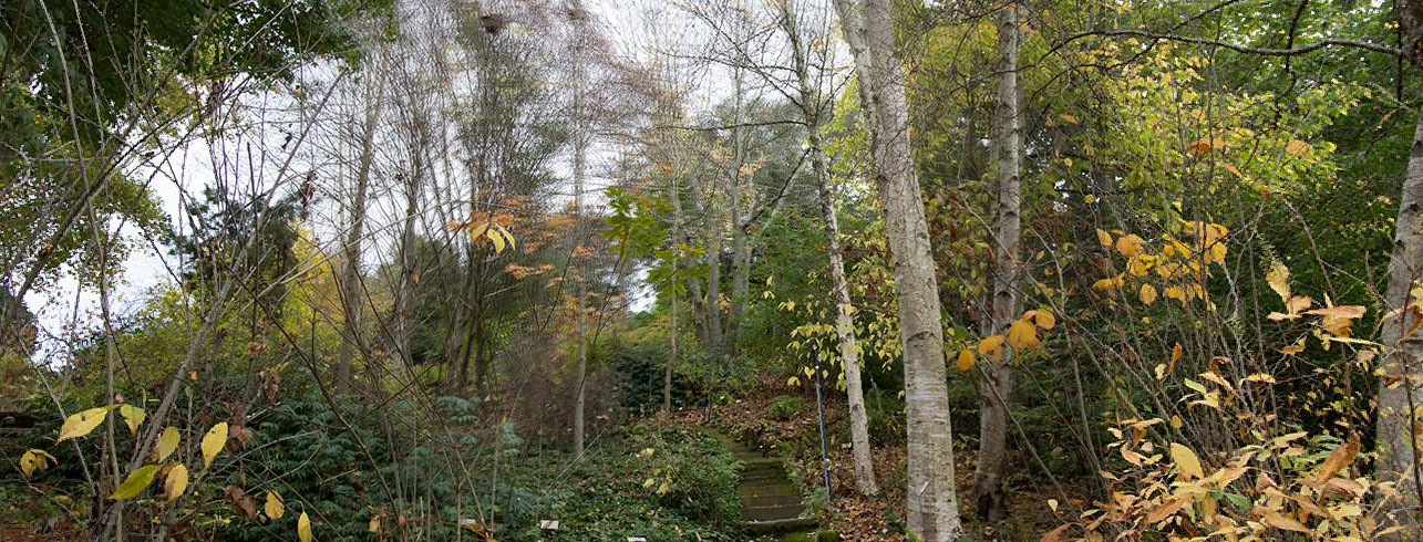
MOSAIC EXAMPLE 2: ASIAN GARDEN
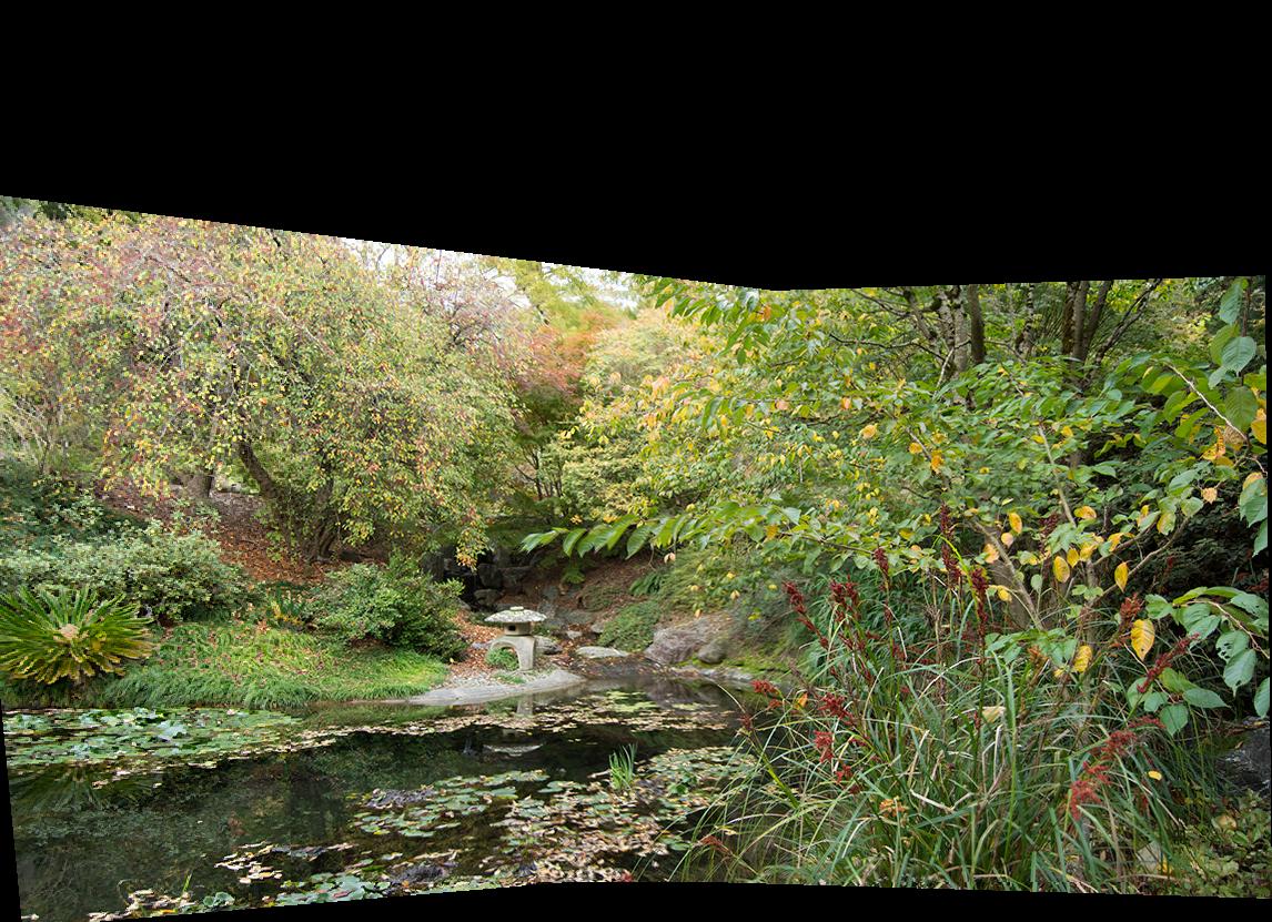
Linear blending
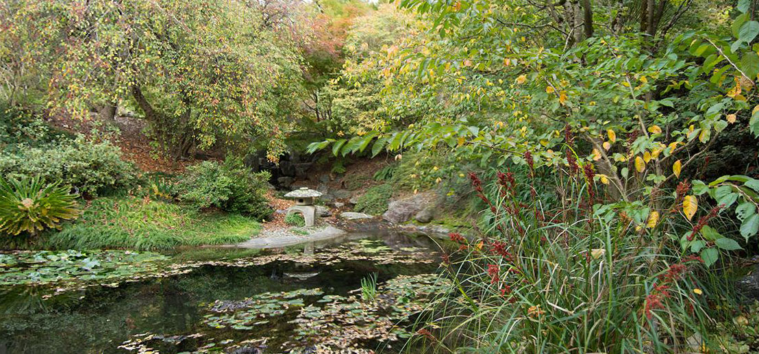
Cropped for aesthetic effect
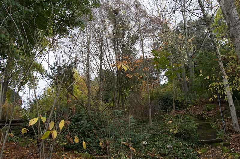
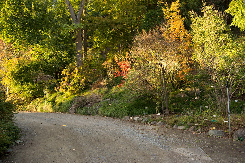
MOSAIC EXAMPLE 3: EASTERN NORTH AMERICA
The mosaic generated from this photoset is actually pretty interesting due to the obvious blurring of the tree branches in the upper portion of the mosaic. This could have been caused by the fact that I selected very few corresponding points in that area due to its being extremely dense and random. Further, there is a noticeable line of darkness at the right side of the mosaic, which is indicative of the overlap between the right and center images. Part of this darkness is likely due to the fact that the brightness in the two original images differs somewhat. The sun was setting behind me at the time that I took these photos, so turning the camera towards my right exposed the lens to more sunlight. This might have caused the camera's auto settings to adjust themselves.
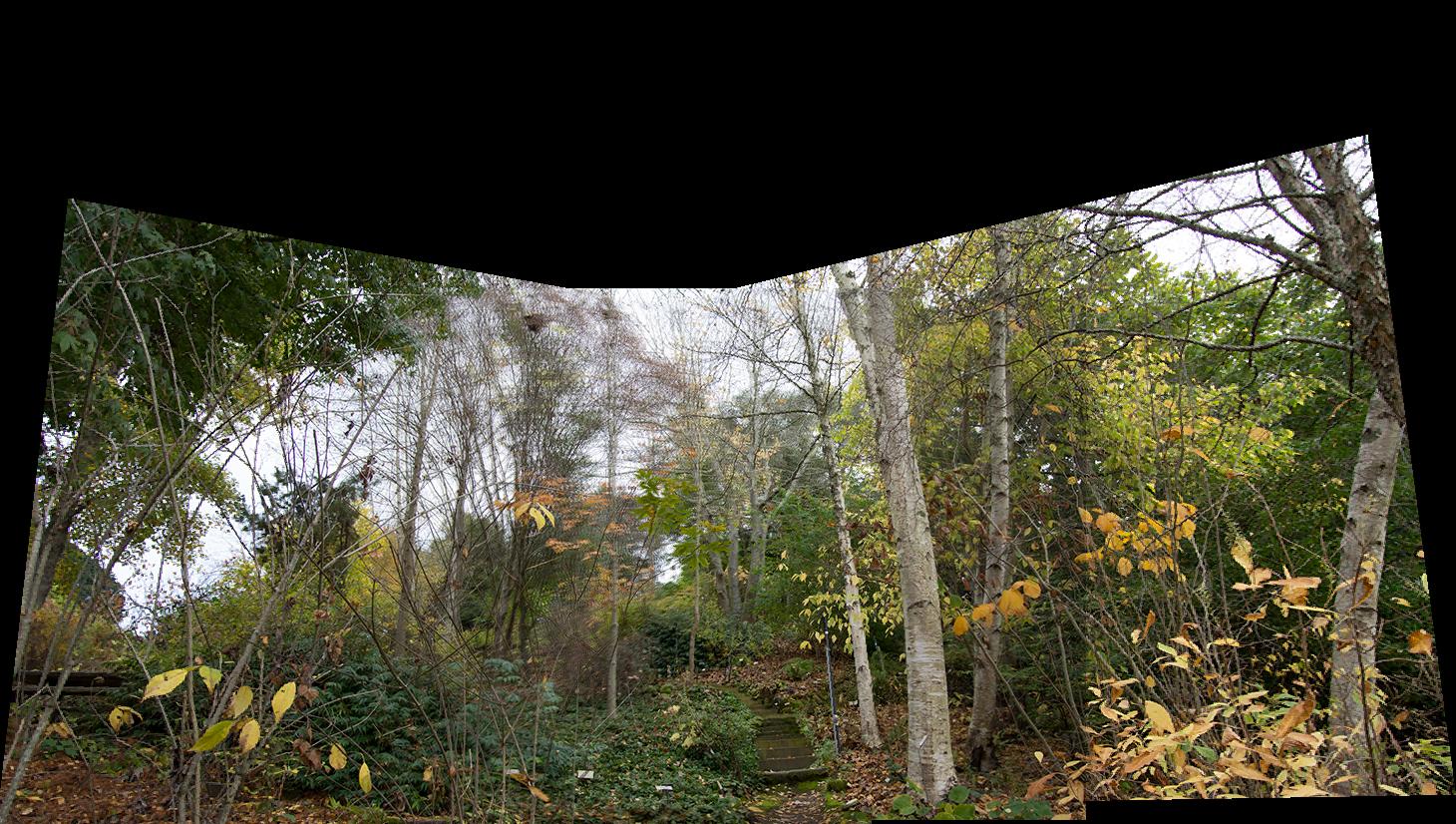
Linear blending
Cropped for aesthetic effect
IV. TAKEAWAYS
Clearly, consistency in photo brightness is really important! Otherwise, no matter what you do, your final image will look odd. Also, foliage isn’t the best subject matter for this technique, as it is unpredictable and may display blurry or odd results. I had to select points more than once for the Asian garden image to get rid of the blurring effect.
PART 2: Autostitching Panoramas
Now that we’ve figured out how to create mosaics from multiple images, let’s figure out how to automate the process (if you haven’t tried it, selecting corresponding points by hand is hard work!). In this project, we roughly follow the process laid out in the paper: Multi-Image Matching Using Multi-Scale Oriented Patches.
HOW TO AUTO-STITCH YOUR IMAGES
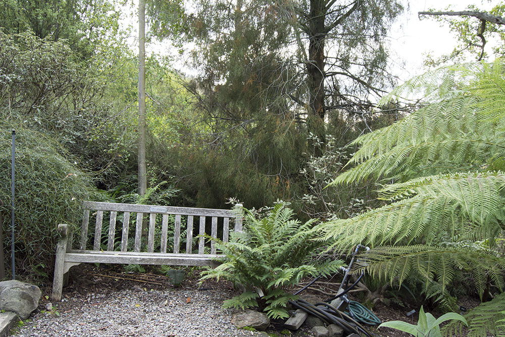
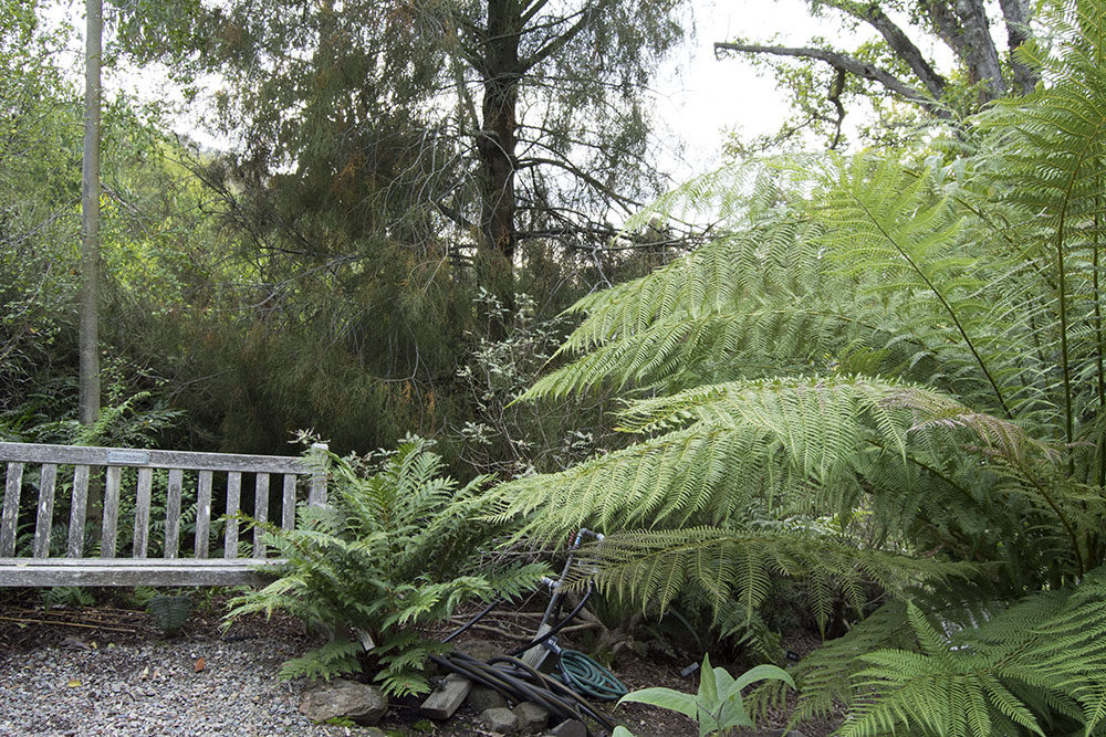
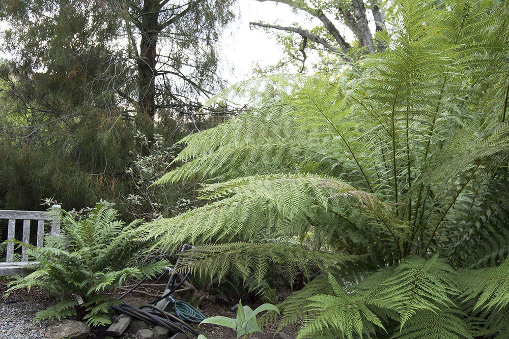
We'll be using the Asian garden image as an example. Here are the original photos. The steps will only be shown for the left and center images.
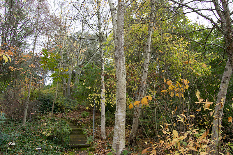
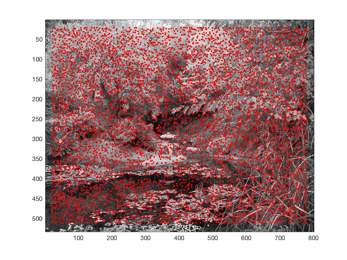
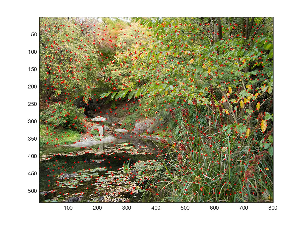
STEP 1: CORNER DETECTION
Detect the corner features of the image. I used the Harris corner detector provided in harris.m.
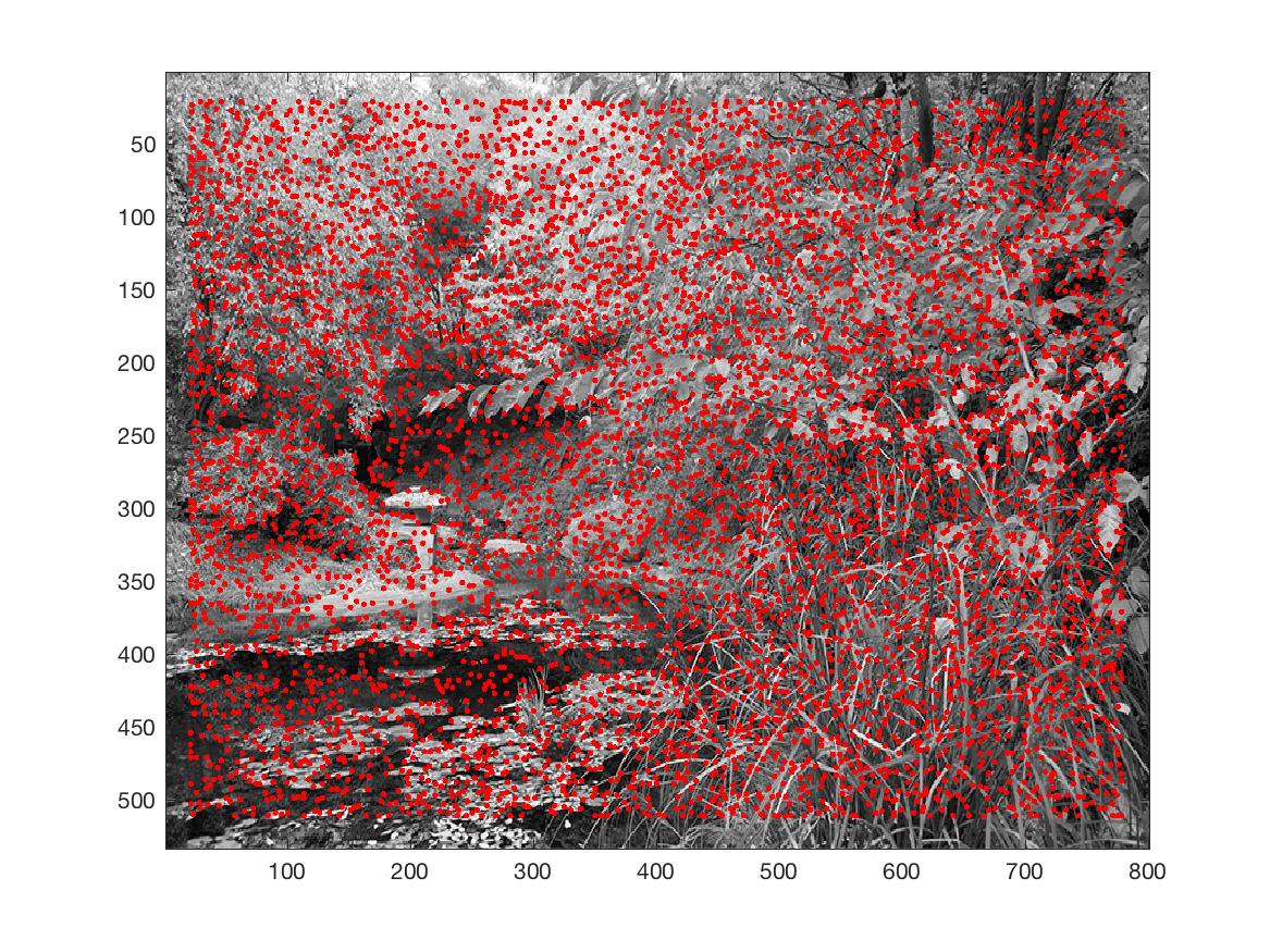
STEP 2: SELECT ONLY THE STRONGEST CORNERS OF THOSE DETECTED
Use the Adaptive Non-Maximal Suppression (ANMS) technique specified in the paper to select a specified number (500, for instance) of corners that are most dominant in their surrounding area. For every Harris corner (xi, yi) in image 1, we calculate its distance from every Harris corner (xj, yj) in image 2.
Let the function f(x, y) give the corner strength for some pixel (x, y).
If f(xi, yi) < 0.9*f(xj, yj) then (xj, yj) is significantly stronger than (xi,yi). In such a case, we compare the distance between (xi, yi) and (xj, yj) to the most recently recorded minimum distance, stored in some variable min_dist. If the new distance is smaller, then it becomes the new value of min_dist. At the end of this process, we sort all points (xi, yi) in img1 by their calculated min_dist information and take the 500 points with the largest min_dist. This means, we’re taking the 500 points that are most dominant in their local areas.
STEP 3: EXTRACT FEATURE DESCRIPTORS
A feature descriptor is a description of the area around a point in an image, the “description” portion really being the pixel values around the central point.
To extract feature descriptors, we, for every ANMS point, sample a 40x40 patch of pixels around the point. We then gaussian blur the patch and downsample it to an 8x8 matrix, after which we do bias-gain normalization by executing: patch = (patch - patch_mean) / std_dev(patch). Finally, we flatten every 8x8 patch into a vector of 64 values.
STEP 4: FEATURE MATCHING
Now, echoing the manual specification of corresponding points that we did in part 1, we need to figure out which ANMS points in img1 match which ANMS points in img2. To do this, we use the features we extracted in step 3, and what Professor Efros calls the “Russian Granny Algorithm.”
For each ANMS point (xi, yi) in img1,
- Calculate the squared Euclidean distance between the point’s feature vector and the feature vector of every single ANMS point in img2.
- Sort the results and select the two points in img2 that have the smallest distance to (xi, yi) and call them nn1 and nn2 (where nn stands for “nearest neighbor”).
- If the ratio nn1/nn2 is smaller than a specified threshold (I used 0.4), then we consider the difference between nn1 and nn2 great enough that we assign the point corresponding to nn1 as our match for (xi, yi).
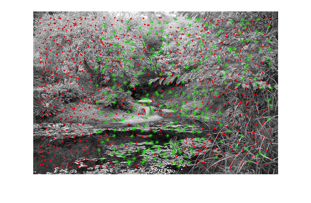
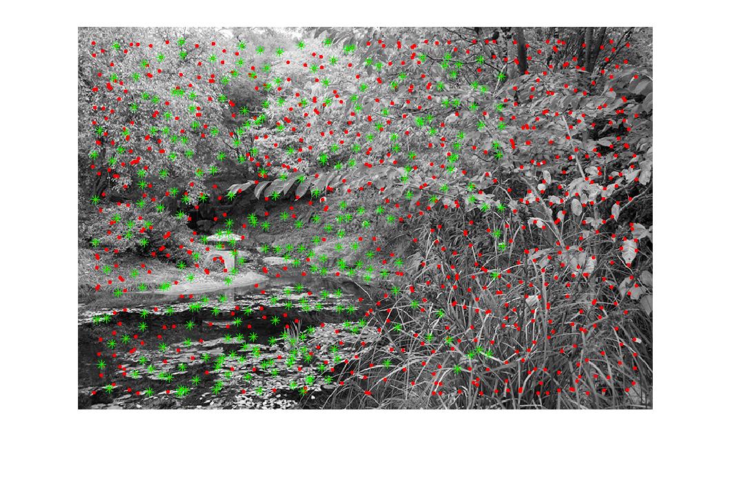
Displayed in green below are points specified by the algorithm to be matches between the left and center images.
Matching points are also calculated between the center and right images.
Left matched to center: Left
Left matched to center: Center
STEP 5: RANSAC FOR COMPUTING HOMOGRAPHIES
Now that we’ve got matched points between img1 and img2, we need to compute the homography between the images. The way we do this is rather straightforward. The following procedure is executed a specified number of times (I used 2000):
We select four random pairs of matched points from our results in step four and calculate a homography based on those points. Then, we apply the homography for for each of the matched pairs from step 4, and calculate the distance from the “converted” point produced by the homography and its matched counterpart. If this distance is less than a certain threshold (I used 1), then the pair is an “inlier” and we consider the homography to have done well for this matched set. We total up the number of inliers for this homography and store it.
At the end of this process, we sort our results and select the homography that got the most inliers.
STEP 6: IMAGE STITCHING
This is simply passing all image information and the homographies calculated from the previous five steps to the functions we wrote in Part 1 of the project. A finished image mosaic will be produced at the end!
Cropped for aesthetic effect
SELECTED AUTO-STITCHED EXAMPLES
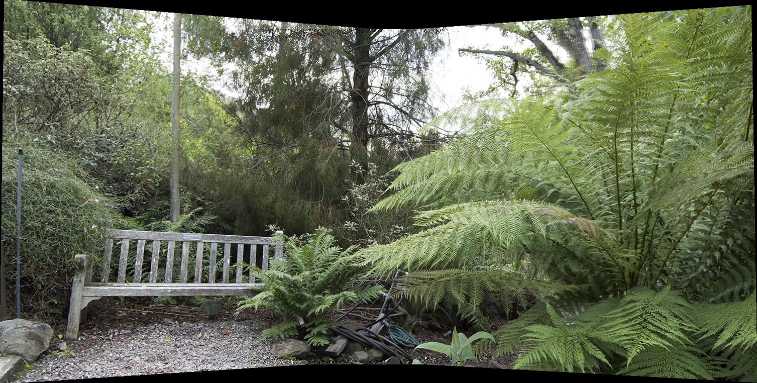
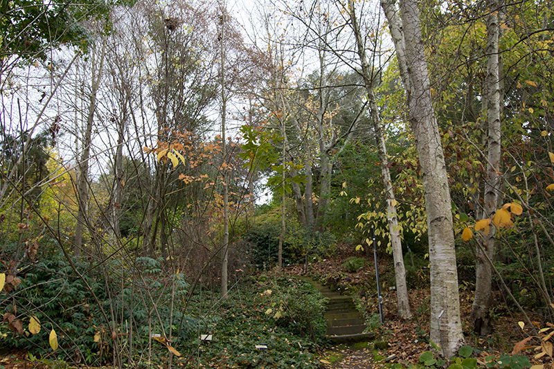
ONE. A bench and North American shrubbery
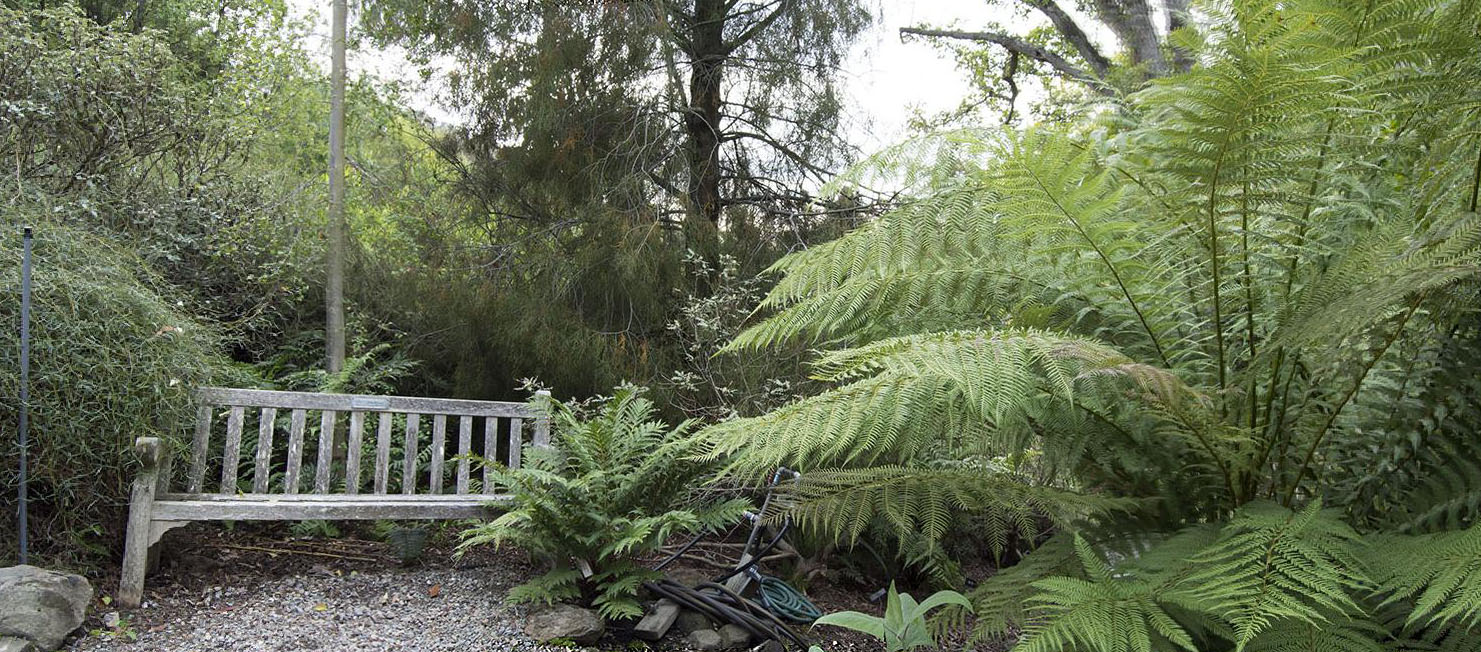
Cropped for aesthetic effect
TWO. Desert ecosystem
Cropped for aesthetic effect
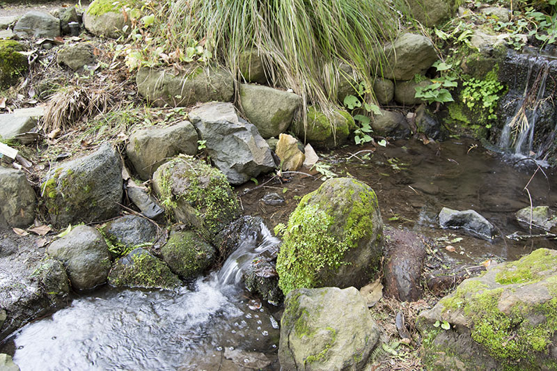
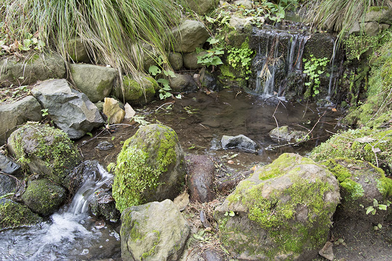
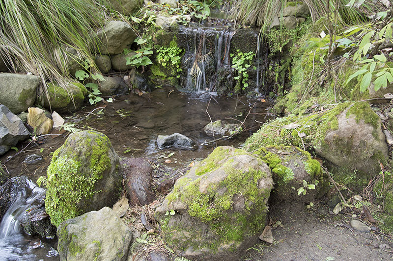
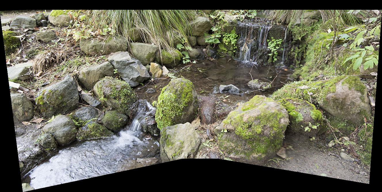
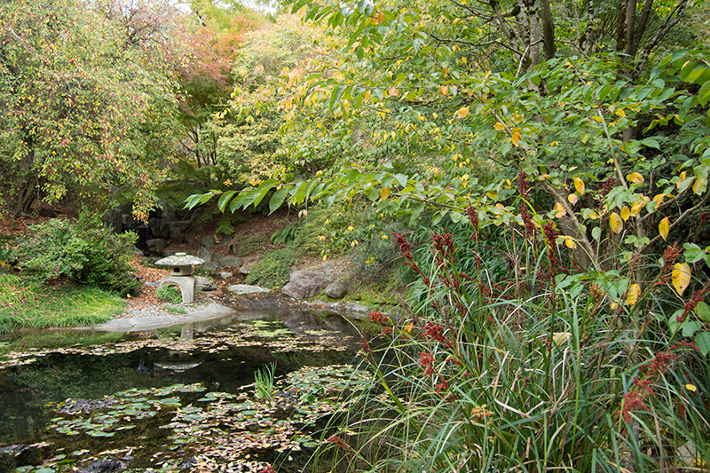
THREE. Little waterfall
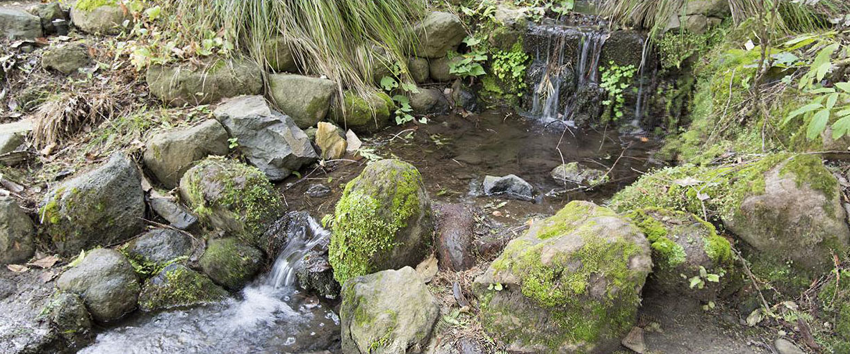
Cropped for aesthetic effect
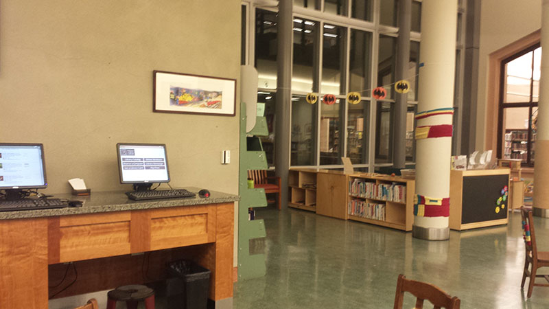
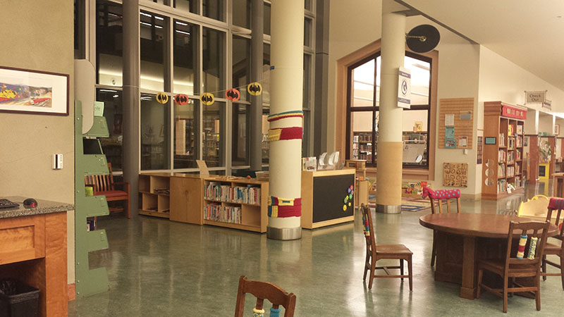
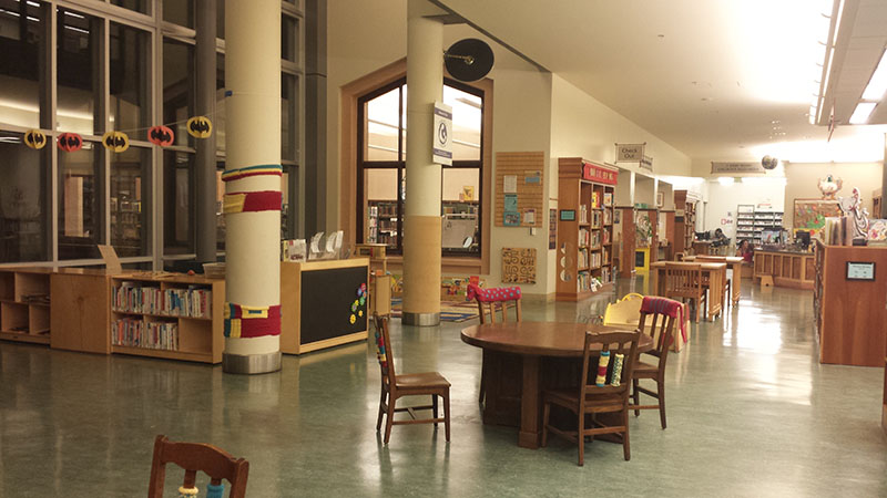
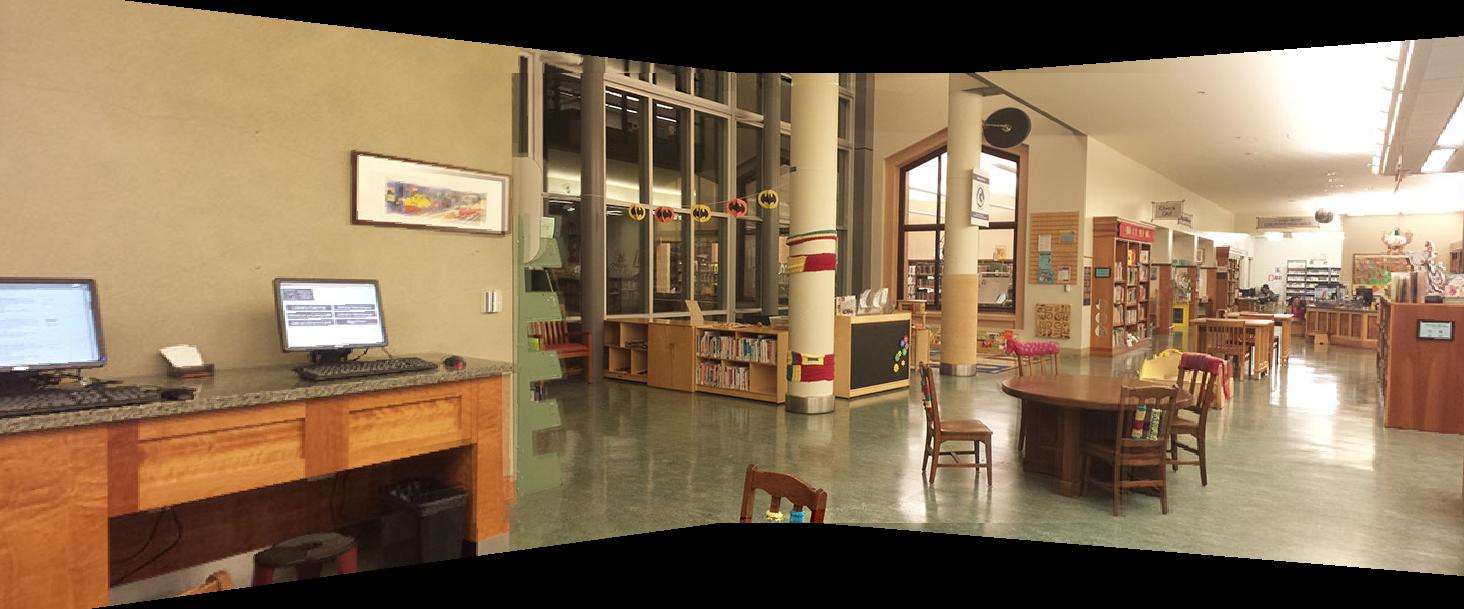
FOUR. The Children's Section of the Berkeley Public Library
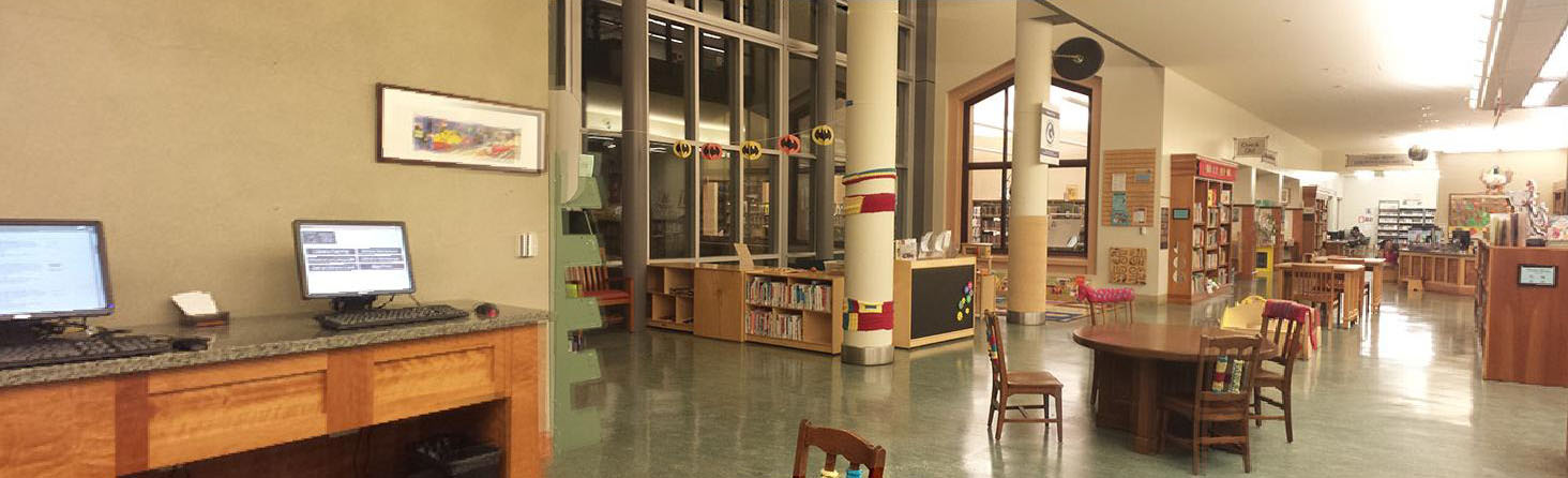
Cropped for aesthetic effect

PANORAMA RECOGNITION
The goal of panorama recognition is to, given a set of unordered images in a directory, figure out which images form panoramas and to stitch them together. My implementation assumes that all mosaics are made of two images only and that all images in the given directory are JPGs.
A surprisingly straight-forward method works quite well in achieving this. I have my program iterate through all the images in the directory and run both Harris and ANMS to select points. I then extract feature descriptors for all of the images.
To figure out which images pair up into panoramas, I run the feature matching algorithm (step 4) on every combination of two image files. If the number of matches found exceeds a certain threshold, then the two images are declared part of the same panorama and are stitched together. I subsequently log that the two images have already been used (to prevent other files from being matched with them).
Since the mosaic-creation function needs to know which image is on the right and which on the left, a bit of checking needs to be done before stitching is possible. I compare the average column position of the matched points in each image. The image with the smaller average column position is the right image and the other the left.
To test my implementation, I put the following six images into a folder, along with a text file:
TAKEAWAYS
This is a practical one that has led to much head-banging in the last few weeks: MATLAB orders everything by column and then row, except in matrix accessing or the size and plot functions, where things are row first and then column!
Having a computer auto-stitch image mosaics is much more efficient and accurate than having a human do the same job. However, these algorithms still have room to grow, as evidenced by the fact that some images work better than others under these techniques. I think it’s amazing that such a simple procedure can obtain such amazing results.